Hello Fellow readers, I have started this blogging journey to entrench myself in the art of expressively articulating experiential comprehension. I am to understand why I 'understand' specific topics by writing about them and explaining them to someone who has never heard of the topic before. For my first article, I have chosen a simple and straightforward concept, but later on I will delve deeper into more complex multifaceted discussions. This in a way is my first test run. Enjoy!
π is not just any typical mathematical constant but has grown to be to be an iconic symbol of mathematics; it has been studied by the human race for over 4000 years. I woke up one day and decided to reinvent π or approximate it in my own way, but with the added modern tools at my disposal. I will calculate the constant π using randomness and by randomness I mean calculating it using the Monte Carlo Method.
The Monte Carlo Method is named after a well known casino town, called Monaco. In a sense, the Monte Carlo Method is about generating random variables to solve a specific problem [1]; it is dependent on the law of large numbers, which has a very central role in probability and statistics. The law of large numbers states that if we independently repeat an experiment quite a number of times and take the average of the results, what we get should be approximately close to the actual value [2]. To remain on the casino theme, if for example a casino has its games rigged for a profitable favour, then one successful win by a customer is not representative of the casino’s loss as the odds are in the casino’s favour. The total net income by the casino will show a profit over a large number of gambling customers, small losses become negligible.
 The city of Monaco
But to get back on topic, how does this help us in calculating π?
Let us set the scene, imagine a 2-dimensional plane with a square and a circle drawn on it. The circle has radius r units and the square has a side of length r. For better comprehension, Let us imagine, in parallel, a game of darts but instead of a Dartboard we will be using a paper with the shapes described above. I am going to be throwing 100,000 darts on this piece of paper and recording where each dart lands.
This can be easily simulated using python. I will be using a pythonic random generator to fill
two arrays with 100,000 random numbers. These two arrays will consist of my X and Y coordinate.
For example, if my arrays looked like this:
X = [3,2,6,5,.....]
Y= [4,7,4,2,.....]
Then my first coordinate will be (3,4) and my second coordinate will be (2,7)...etc.
x_arr = randint(-10.0, 10.0, 1000000)

y_arr = randint(-10.0, 10.0, 1000000)
After generating my X and Y coordinates, I will check if they are inside my circle or square. In real life, checking whether the darts landed in a circle or the square or neither would be a simple matter of seeing. But in a computer algorithm we need to take more mathematical steps. I will be using the geometric equation of the circle to determine whether the coordinates fall inside the circle or not.
Since my circle will be centered around the origin—or coordinate (0,0)— My equation will be `x^2 + y^2 = r^2` , my r in this case will be equal to 3. Hence, the circle's equation will be `x^2 + y^2 = 9`. To check if a coordinate is within a circle or not, I will simply substitute the x and y values to those of the coordinates’. If let’s say my coordinates are (2,3) then by substituting for the equation I get: `(2)^2 + (3)^2` which equals 13. Since 13 is greater than 9 then the coordinate is outside my circle. If the value is less than or equal to 9, then it is inside my circle. For my square, I will be setting it’s coordinates to (-4,3), (-7,3), (-4,6), (-7,6). I will check if the coordinate is inside the square by simply checking if its X values are less than -4 and greater than -7 and their Y values must be greater than 3 and less than 6.
    for i in range(1000000):

           val = x_arr[i]**2 + y_arr[i]**2

           if(val < 9):

                  circ_counter = circ_counter+1

           elif((x_arr[i]< -4) and (x_arr[i]>-7 )and (y_arr[i]>3) and (y_arr[i]<6)):

                  sqr_counter = sqr_counter+1
 A game of darts
I have set up counters which will show the number of darts that fall within the circle or the square. After 100,000 darts I am ready to calculate π. However, I would like us to remember the concept of areas. It is easy to state the equations of the areas and know them by heart, but in our case we need to understand that the area is the sum of all points within a specified parameter. In simpler terms, we are measuring how much surface is within a specific section. The surface of this section is made up of points or dots. In our case, we randomly filled a circle with darts, the accumulation of these darts —or the amount of surface they cover— will approximately equal to our areas.
The number of darts in the circle ~ the area of a circle = `π * r^2`. The number of darts in the square ~ the area of the square =`r^2`.
So if we divide the number of darts within the circle by the number of darts within a square or
`(π * r^2) / r^2` , what we get is an approximation of π.
I will add the following lines of code to my previous for-loop
if(sqr_counter!=0):

            error_g[i] = (circ_counter/sqr_counter)/2
To get better answers, I will repeat the aforementioned calculations 100 times, each repetition with different randomly selected coordinates. I will thereafter average all of my approximated πs and the average will be our final answer.
Final loop will look like this:
n = 100 #number of times that my simulation will be run

val1=np.zeros(n)

error_g = np.zeros(1000000)

for w in range(n):

        circ_counter = 0

        sqr_counter = 0

        x_arr = randint(-10.0, 10.0, 1000000)

        y_arr = randint(-10.0, 10.0, 1000000)

        for i in range(1000000):

             val = x_arr[i]**2 + y_arr[i]**2

             if(val < 9):

                  circ_counter = circ_counter+1

             elif((x_arr[i]< -4) and (x_arr[i]>-7 )and (y_arr[i]>3) and      v(y_arr[i]<6)):

                  sqr_counter = sqr_counter+1

            vif(sqr_counter!=0):

                 verror_g[i] = (circ_counter/sqr_counter)/2

         val2 = circ_counter/sqr_counter

         val1[w]= val2/2
There, ladies, gentlemen, and variations thereof, we have calculated π using randomness.
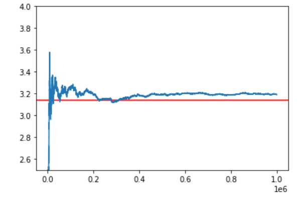
The interesting part of it all was how the approximate values approach π with the addition of
each coordinate. The more coordinates I added to my calculations the more it converged to the
value of π. Below you can see how our values fluctuate and then converge to the value of π —
represented by the red line.
The code to illustrate that is a part of the overall code I showed above, I then used
matplotlib.pyplot library to plot the following line graph:
Code for this is:
plt.axhline(y=np.pi, color='r', linestyle='-')

plt.plot(error_g)

plt.ylim(2.5, 4)

plt.show()
you can check out the entire code out on GitHub
Thank you for reading, if you have any questions you can contact me through the main page at Anton Kopti.